Check out the git repo!

Molecular Dynamics Method and the Lennard-Jones Potential

This is a method in which the evolution with time of a system of interacting particles is modelled by integrating their equations of motion. We represent the forces of interaction between the particles as a gradient of the potential energy of the system. In our case: the Lennard-Jones potential, which, despite being one of the simplest, is the one that has been studied most extensively.

$$ U(r_{ij}) = \begin{cases} \displaylines{4 \varepsilon \left[ \left( \frac{\sigma}{r_{ij}} \right)^{12} - \left( \frac{\sigma}{r_{ij}} \right)^6 \right] + \varepsilon, & r_{ij} < r_c = 2^{1 / 6} \sigma \\ 0 & r_{ij} \ge r_c} \end{cases} $$

$$ f = - \nabla U(r) $$

Maxwell Distribution of Velocities' Projections

Distribution of velocities' projections in logarithmic scale. The deviation from a straight line at the end is due to the fact that our system has only a finite number of particles, and the Maxwell's distribution is true for a infinite amount.

2 Methods for Calculating the Self-Diffusion Coefficient

1. Einstein's Relation

$$ D = \frac{1}{2 N d} \frac{1}{t} \left\langle \sum_i \left[ \vec{r}_i(t_0 + t) - \vec{r}_i(t_0) \right]^2 \right\rangle $$ where $d = 3$ - dimensions, $N$ - number of particles, $\vec{r}_i(t)$ - coordinate vector of the $i$-th particle at time $t$.

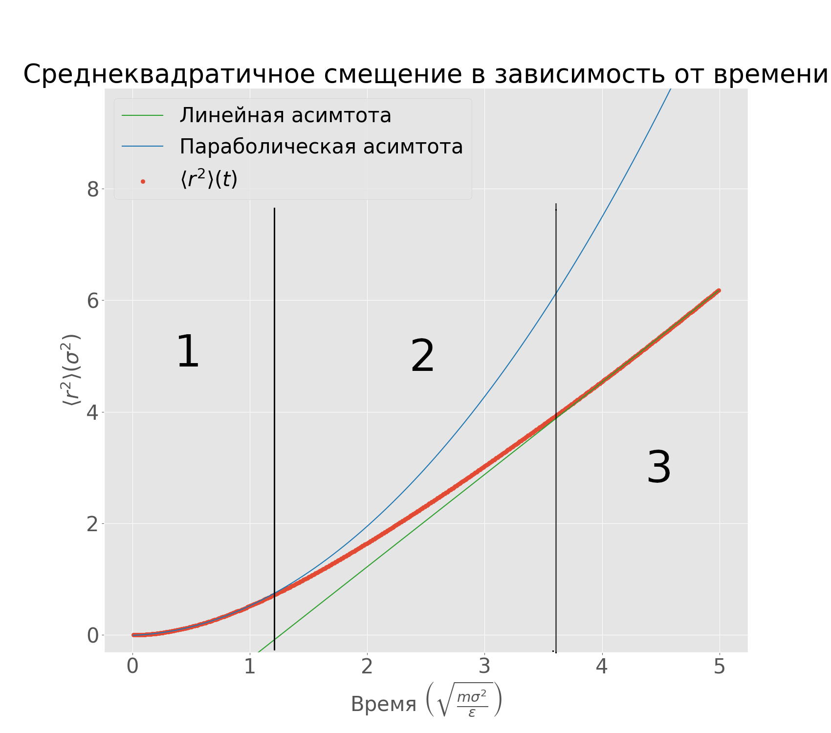
Mean squared displacement.

The x axis corresponds to time, and the y axis to the mean squared displacement, both in Lennard-Jones units. In green: linear asymptote, and in blue: parabolic asymptote.

By taking into account only the linear segment, and with the help of the least squares method, we fit it to a straight line. The scope of the line is equal to the diffusion coefficient multiplied by 6, or $6D$.

2. Effective Diameter of Collision

Let's consider the interaction between two molecules. We want to know $r_0$ - the closest distance they can reach. Let them go towards each other along their central lines with an initial relative speed $v_{12}$. Their initial kinetic energy gradually turns into potential energy until they reach $r_0$, which is the turning point, where $$ \frac{1}{2}m v_{12}^2=4\varepsilon\left(\frac{\sigma}{r_0}\right)^{12} $$

This way we can calculate the effective diameter of collision.

The effective gas-kinetic cross section $$ q = \pi r_0^2 $$

The mean free time $$ \tau = \frac{1}{\sqrt{2}n\langle v \rangle q} =\frac{1}{\sqrt{2}n\langle v \rangle \pi r_0^2} $$

Now let's estimate the free path time using the plot $\langle r^2 \rangle (t)$. Let's use a double logarithmic scale, and extrapolate the linear and parabolic fits. Their intersection gives and estimate on $\tau$ - the mean free time.

The diffusion coefficient can be approximated $$ D = \frac{1}{3} \langle v \rangle \ell $$ where $\ell$ is the mean free path.

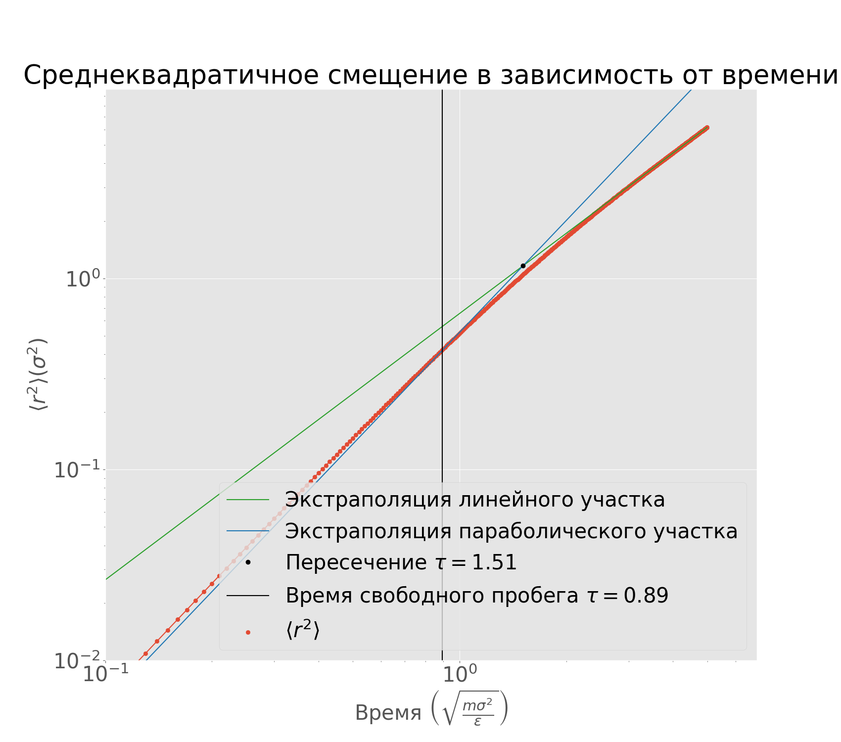Mean free path in relation to time in double logarithmic scale. We extrapolate the linear and the parabolic segments and their intersection is an estimate for the mean free time.

Results

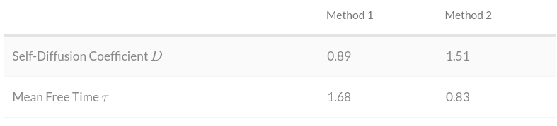
Conclusion

By numerically solving Newton's equation, we obtained the Maxwell velocity distribution and the diffusion law. Molecular kinetic theory gives and acceptable fit.

We also checked the limits of application of the molecular dynamics method with the Lennard-Jones potential.

It is known that the mean free path cannot be determined exactly. Therefore, given that the values obtained differ from each other by a factor of $2$, we can conclude that they coincide within these limits.

Since we calculated the same value using two different methods, and they coincide, we can conclude that our model works correctly and we successfully calculated the gas diffusion coefficient using the molecular dynamics method.