Check out the git repo!

Application of the Markov Chain Monte Carlo Method in scattering problems

In scattering problems, the motion of a particle in a medium consists of a rectilinear motion between collisions if the trajectory is not bent by the action of an external field, and the actual acts of scattering on particles of the environment. In our model, scattering leads to instantaneous change in the velocity vector of the particle, its kinetic energy, internal state (excitation of internal degrees of freedom), as well as analogous changes in the parameters of the medium particle. For all the listed variables, the corresponding distribution functions of probability must be known. Here we will only consider the two main components of scattering: the change in the velocity vector and the time between collisions.

Simulating the Time Between Collisions

We use the following model to find the probability density for a particle to travel a path of length $\ell$ before collisioning. Let a parallel beam of particles with intensity $I_0$ fall into a medium with a mean free path $\lambda$. The boundary of the medium is at length $\ell = 0$.

The mean free path $$ \lambda = \frac{1}{N \sigma_m} $$ where N is the particle density of the medium, and $\sigma_m$ is the transport cross section of scattering f incident particles on particles of the medium, which describes the scattering process.

Particles that have undergone a collision are consider to have left the beam. We can use a differential equation to describe the decrease in the intensity of the beam $dI$ due to collisions after passing a distance $d\ell < \sigma_m$ $$ dI = -I(\ell) \frac{dI}{\lambda} $$

The solution: $$ I(\ell) = I_0 \exp \left( -\frac{\ell}{\lambda} \right) .$$

The probability of a collision when passing a distance from $0$ to $\ell$, or the distribution function, is equal to $$ F_\ell(\ell) = 1 - \exp \left( -\frac{\ell}{\lambda} \right) $$ and the probability density of particle scattering along the path $\ell$ is $$ p_\ell(\ell) = \frac{dF_\ell}{d\ell} = \lambda^{-1} \exp \left(-\frac{\ell}{\lambda} \right) $$

The mean free path $$ \left\langle \ell \right\rangle = \int_0^\infty \ell p_\ell(\ell) d\ell = \int_0^\infty \frac{\ell}{\lambda} \exp \left( -\frac{\ell}{\lambda} \right) = \lambda $$

$$ \left\langle \ell^2 \right\rangle = \int_0^\infty \ell^2 p_\ell(\ell) d\ell = \int_0^\infty \frac{\ell^2}{\lambda} \exp \left( -\frac{\ell}{\lambda} \right) = 2 \lambda^2 $$

The sequence of mean free paths has the following form $$ \ell = -\lambda \ln (1 - r) $$ where $r$ is a random number, with an uniform distribution on $(0, 1)$.

The time $\tau$ between collisions is obtained by dividing the above equation by the relative velocity of colliding particles $v_{rel}$ $$ \tau = - v_m^{-1} \ln(1 - r) $$ where $v_m = N \sigma_m v_{rel}$ is the collisions frequency.

Simulating the deviation angles of the velocity vector

The probabilily of a particle scattering by an angle $\theta$ in the center-of-mass system of colliding particles is determined by the differential scattering cross section $\sigma(\theta, v_{rel})$. The conversion to the laboratory frame of reference can be obtained from kinematic relations or from a textbook, for example, "Mechanics" by Evgeny Lifshitz and Lev Landau.

The laboratory coordinate system practically coincides with the center-of-mass system if the mass of the scattering particle is much less than the masses of the particles of the medium, for example, in the case of the scattering of an electron beam in an atomic-molecular medium. Let's assume this is the case we are considering.

Deviation of the velocity vector is characterized by two angles: the angle $\theta$ in the plane of collision and the angle $\varphi$ direction of the velocity vector before the collision. Let's introduce the vectors $\mathbf e$ and $\mathbf e$ as unit velocity vectors before and after the collision.

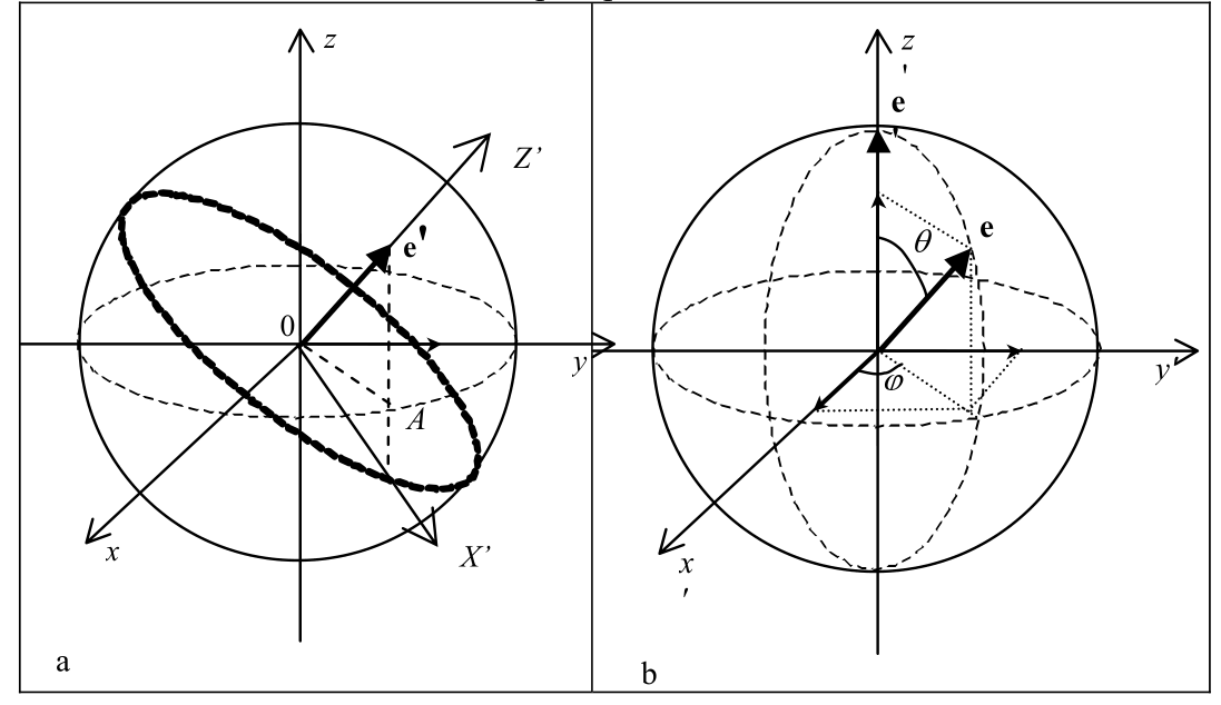
In case of a collision of two structureless particles, thanks to the conservation of angular momentum, the particles move in one plane. Therefore, at a given collision velocity, the scattering cross section depends only on angle $\theta$ and not on $\varphi$. The angle $\varphi$ determines the position of the collision plane in space.

The probability of scattering into a solid angle $d\Omega$, by definition of the scattering cross section, is equal to $$ p(\theta, \varphi) d\theta d\varphi = \frac{\sigma(\theta) d\Omega}{\int_0^{4\pi} \sigma(\theta) d\Omega} $$

$$ p(\theta, \varphi) d\theta d\varphi = \frac{\sigma(\theta) \sin\theta d\theta d\varphi} {2\pi \int_0^{\pi} \sigma(\theta) \sin\theta d\theta} $$

Since the scattering cross section is independent of the angle $\varphi$ the probability density decomposes into the product of independent probability densities

$$ p_\theta(\theta) = \frac{\sigma(\theta) \sin \theta} {\int_0^\pi \sigma(\theta) \sin \theta d\theta} $$

$$ p_\varphi(\varphi) = \frac{1}{2\pi} $$

We will look at the case of isotropic scattering, so $\sigma(\theta) = const$.

$$ F_\theta(\theta) = \frac{\int_0^\theta \sigma(\xi) \sin\xi d\xi} {\int_0^\pi \sigma(\theta) \sin\theta d\theta} = \frac{1 - \cos\theta}{2} $$

Therefore, the Markov sequence of scattering angles will be determined by the formula $$ \cos \theta = 1 - 2r $$ where $r$ is once again a random number uniformly distributed on the segment $(0, 1)$.

$$ \varphi = 2\pi r $$

Calculating the Particle Displacement

The displacement of the particle after a collision can be described by $$ \Delta x = a\ell, \: \Delta y = b\ell, \: \Delta z = c\ell $$ $$ a^2 + b^2 + c^2 = 1 $$

Here $\ell$ is determined by the formula, which we derived earlier $$ \ell = -\lambda \ln(1 - r) $$

Since we describe the change in the velocity vector using angles of deviation from the previous direction, and not with coordinates, we need to establish their connection. The solution of the corresponding trigonombric program gives the following solution.

If $|c'| \ne 1$ $$ a = \mu a' - (b' \sin\varphi - a'c' \cos\varphi) \sqrt{\frac{1 - \mu^2}{1 - c'^2}}, \mu = \cos \theta $$

$$ b = \mu b' + (a' \sin\varphi + b'c' \cos\varphi) \sqrt{\frac{1 - \mu^2}{1 - c'^2}} $$

$$ c = \mu c' - (1 - c'^2) \cos \varphi \sqrt{\frac{1 - \mu^2}{1 - c'^2}} $$

If $|c'| = 1$ $$ a = \sin\theta \cos\varphi $$ $$ b = \sin\theta \sin \varphi $$ $$ c = \cos \theta $$

Results

1. Distribution Function

The simulated process is the electron diffusion from a point source in a noble gas characterized by the electron mean free path $\lambda = 1$. We assume that the electron energy is less than the threshold for excitation of the internal states of the medium particles, and we neglect the elastic energy losses in the collision of an electron with an atom.

Also, electron scattering on the atoms is considered isotropic.

The distribution of particle positions at different moments in time.

Calculation of the Diffusion Coefficient

We verify the Stokes-Einstein law for diffusion.

$$ L = \sqrt{6Dt} $$

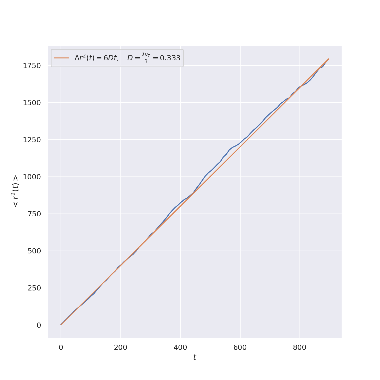Graphic depiction of the dependence on time of the length $L$ of the electron displacement vector from he starting point and the theoretical dependence according to the Einstein formula.

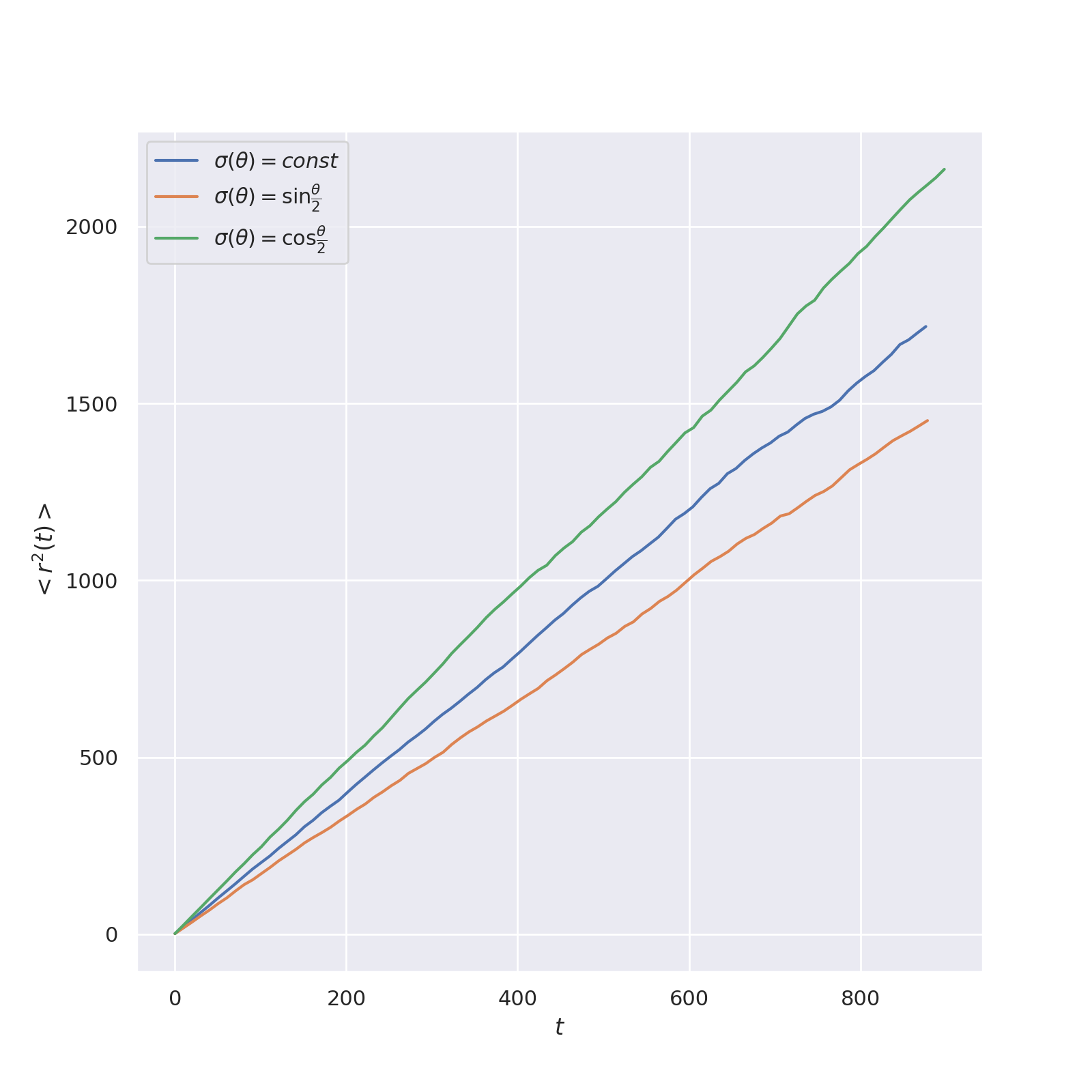
MSD for Different Differential Electron-Scattering Cross Sections

We calculate the mean square displacement for different values of differential scattering cross sections:

1. $\sigma(\theta) \propto \sin \left( \frac{\theta}{2} \right)$

$$ F_\theta(\theta) = \frac{\int_0^\theta \sigma(\xi) \sin\xi d\xi} {\int_0^\pi \sigma(\theta) \sin\theta d\theta} = \frac{\int_0^\theta \sin \left( \frac{\xi}{2} \right) \sin\xi d\xi} {\int_0^\pi \sin \left( \frac{\theta}{2} \right) \sin\theta d\theta} = \frac{\frac{4}{3} \sin^3 \left( \frac{\theta}{2} \right)} {\frac{4}{3}} = \sin^3 \left( \frac{\theta}{2} \right) $$

2. $\sigma(\theta) \propto \cos \left( \frac{\theta}{2} \right)$

We compare the results obtained with the case of isotropic scattering.

Comparison of different values of the scattering cross section.

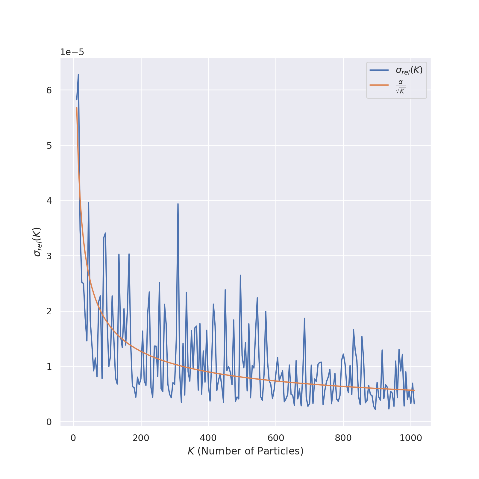
Error Analysis

We verify that the error of the method is $ \propto \frac{1}{\sqrt{K}}$, where $K$ is the number of electrons.

Literature

1. Monte Carlo Method. Teaching aid on the course Computational Methods of Experimental and Theoretical Physics. V. R. Solovyov.

2. Monte Carlo. Sobol I.M. 1985

3. Gould, H. and J. Tobochnik, 1988, "An Introduction to Computer Simulation Methods. Applications to Physical Systems."

4. 3. Elkin N.N. Course objectives: fundamentals of computational physics. MIPT. 1999.